Visualizing different levels of the brain atlas structure hierarchy graph in Neuroglancer
Brain atlases, such as the Allen Mouse Brain Atlas (AMBA) and Princeton Mouse Brain Atlas (PMA) are invaluable tools. They allow data from different experiments to be compared and analyzed in the same framework. With Neuroglancer and other visualization tools, they allow data to be visualized in the same framework as well.
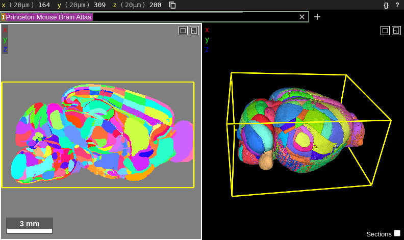
The way we visualize these atlases with Neuroglancer is by showing their atlas annotation volume. Described here for the AMBA, the annotation volume is a 3D volume containing ids at voxels corresponding to the locations of brain regions. Each id represents a different brain region. When the Allen Brain Institute created their annotation volume, they had to choose what level of brain divisions to use. For example, did they want to display only the very large brain divisions like Cerebral Cortex, Cerebellum and Brain Stem, or the more detailed subdivisions such as the nuclei contained within these larger regions? Allen largely chose the latter option, which is why their annotation volume has so many small regions:
But what if the researcher wants to display larger brain divisions for a figure they are making? Fortunately, we are not stuck with visualizing the atlas only at the brain divisions that Allen chose. To figure out how to overcome this, we need to understand the atlas structure hierarchy (sometimes referred to as the “brain ontology” or “structure ontology”). The structure hierarchy is a set of parent-child relationships describing how the large and fine divisions of the brain are related. They are nicely visualized using directed graphs. For example, here is the structure hierarchy graph for the Striatum, a brain region situated beneath the cerebral cortex in the mammalian brain that is critical for many cognitive functions. Hover over the image to zoom. Clicking the image will open it in its own window.
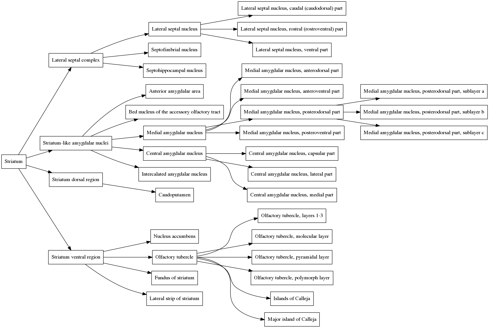
In the graph, the Striatum is the parent node (all the way to the left). It is composed of four smaller regions, the Lateral septal complex, the Striatum-like amygdalar nucleus, the Striatum dorsal region and the Striatum ventral region, all of which are connected to the Striatum by edges in the graph. Each of these subregions is composed of its own set of subregions, which themselves have subregions, and so on. The entire brain can be organized in this way, and the structure hierarchy defines all of these relationships. The graph of the structure hierarchy of the entire mouse brain is massive and impractical to show on this page, but we don’t need it to understand how the structure hierarchy is organized.
So what we need to do in Neuroglancer if we want to show larger brain divisions than Allen’s defaults is to modify the structure hierarchy that the annotation volume is using. I created a key binding in Neuroglancer that allows users to do exactly that. One key (“p” for parent) allows users to go up a level in the hierarchy, and another key (“c” for child) allows them to go in the opposite direction. It makes use of Neuroglancer’s segment equivalences feature by merging children with their parents so they have the same color and id. Here is a video example showing these key bindings in action for the Striatum. At the beginning of the video, the default structure hierarchy of just the Striatum is displayed, corresponding to the graph shown above. The “p” key is pressed three times, showing the structure hierarchy collapsing to larger and larger divisions until the entire Striatum is shown as a single region. At the end of the video, the “c” key is pressed and the original divisions are restored.
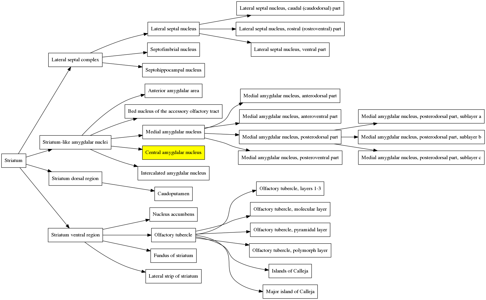
Here is the an illustration of what is happening in the structure hierarchy graph when the atlas is contracted in the video above. Immediately before the atlas is contracted the first time, the cursor is on the brain region: “Central amygdalar nucleus, capsular part”, which is highlighted in the graph below to show which branch we are in.

When the atlas is contracted the first time, this region and its siblings are merged with the parent region, the “Central amygdalar nucleus”. That branch in the structure hierarchy graph therefore gets one level smaller and is now:
When the atlas is contracted a second time, all of the siblings of the “Central amygdalar nucleus” and all of their descendants get merged with the parent, the “Striatum-like amygdalar nuclei”, and the graph becomes much simpler:
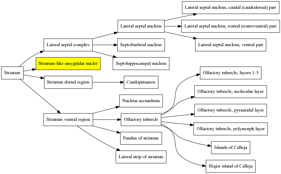
And finally when the contraction is performed again, the entire structure collapses back to the Striatum because the “Striatum-like amygdalar nuclei” is a child of the Striatum and therefore all of its siblings are also children of the Striatum. So the graph simply becomes:

At the end of the video the “c” key is pressed and the original structure hierarchy of the Striatum is restored.
A jupyter notebook walking through how I created these graphs and the Neuroglancer add-on is available here: https://github.com/PrincetonUniversity/lightsheet_helper_scripts/blob/master/neuroglancer/merge_ontology_tutorial.ipynb
Try out the tool yourself in this live demo (only available within the Princeton network of VPN): https://braincogs00.pni.princeton.edu/neuroglancer/merge_ontology_demo