Verpeut et al. Y-maze c-Fos brain samples
This page contains links to interactive visualizations of brain-wide c-Fos expression and cerebellar injection site localization from mouse subjects studied in the manuscript “Cerebellar contributions to a brainwide network for flexible behavior” by Jessica L. Verpeut et al. (pdf: https://www.biorxiv.org/content/10.1101/2021.12.07.471685v1). Treatment groups are listed in bold, and links are for individual subjects. Only treatment groups CNO Crus I Left, CNO Crus I Right, Crus I Bilateral Reversal, and Lobule VI Reversal contain injections. In those cases, a separate “(injection)” link appears beside each c-Fos link. Any subjects with the prefix “dadult” have neither injection links nor an atlas layer (see below) due to the fact that the cerebellum was removed from the rest of the brain before imaging. c-Fos expression is still visible in those brains, however.
Neuroglancer How-to
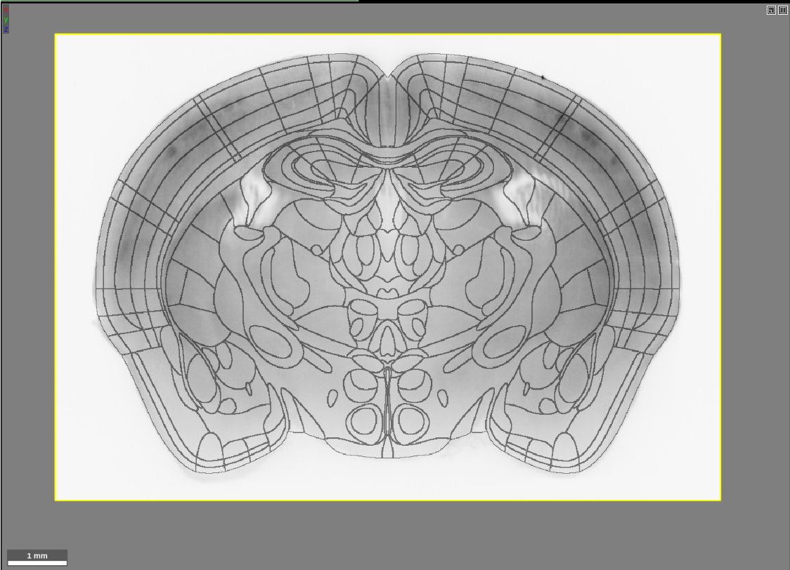
The visualizations at the following links use the web application Neuroglancer for displaying and interacting with the data. Neuroglancer displays datasets in “layers”, each being represented by a text box near the top of the screen. The figure below shows what the top half of the screen will look like upon clicking the link an19 (c-Fos) in the CNO reversal (control) group section below.
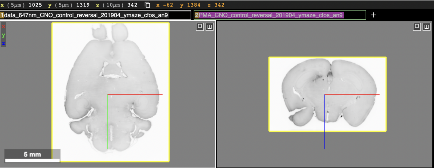
At the very top, the current position within the brain volume along with the physical scale of the dataset are shown. Below that are the layer boxes, “data_647nm_CNO_…” and “PMA_CNO_…” The first contains the brain tissue and the second the Princeton Mouse Brain Atlas (PMA) which has been aligned to the brain tissue (not shown in the figure). Below the layer boxes are the viewer panels. In the figure above the horizontal (left) and coronal (right) sections of the same brain tissue are shown. The sagittal view (not shown in the figure) is displayed in a lower right panel in Neuroglancer. The 3D view, which can be ignored for this dataset (not shown in the figure) is displayed in the lower left panel in Neuroglancer. There is also an x,y,z coordinate axis (blue, red, green lines) that indicates the center of both views. It can be used to determine the relative orientation between the two views.
In the above figure, the brain atlas layer is toggled off by default, indicated by the strikethrough text in its layer box. To toggle on the brain atlas, click the text box where the strikethrough text is shown. Upon doing that, the top half of the screen will now look like this:
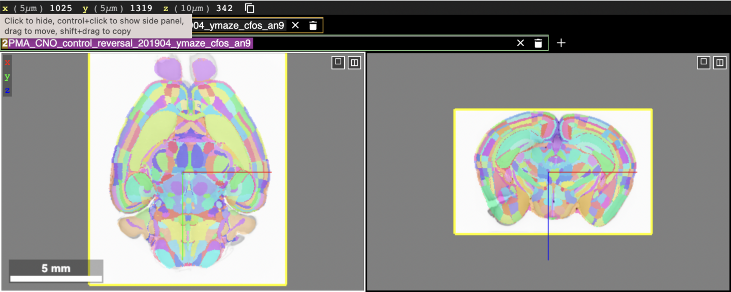
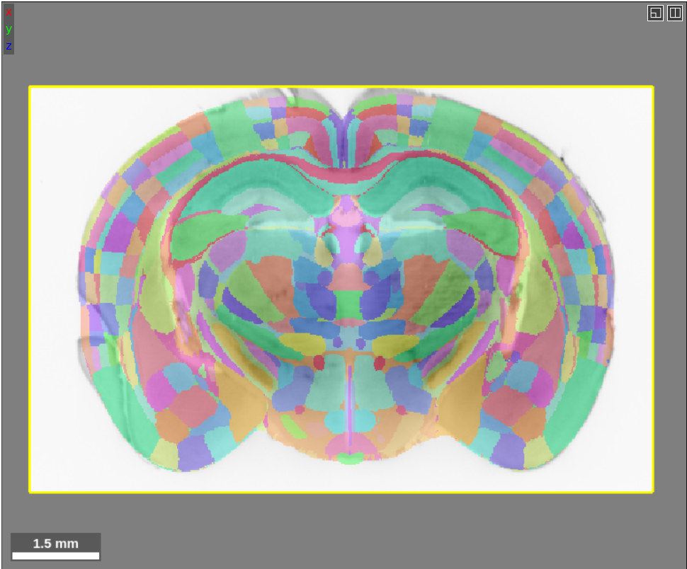
The aligned brain atlas regions are now shown on top of the brain tissue. They are multicolored so that the boundaries between regions can be distinguished. Hovering over a brain region will display the name of the region in the atlas in the layer text box for the atlas. The atlas layer can be made more transparent so that the brain tissue underneath can be seen more easily. This can be done by selecting the “Render” tab on the right hand side panel (not shown in figure but will be displayed in Neuroglancer) and adjusting the opacity slider.
The injection links below have a third layer, which shows the segmented area from the injection site we detected using a program for analysis. The following figure shows what those links will look like:
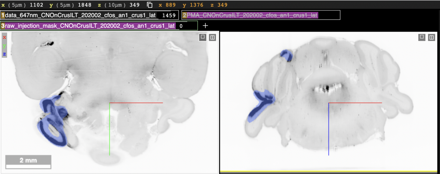
The first two layers “data_647nm_…” and “PMA_CNO…” have the same layout as before (but for a different subject), where the brain atlas layer (second layer) is toggled off by default. The third layer, “raw_injection_mask_…” is new. This layer is shown as the blue area in the viewer panels.
Neuroglancer has some basic keystroke commands that enable you to explore the multidimensional data:
- h key: open help menu
- (2D view) left-click and drag: translate section
- (2D and 3D view) mouse-wheel: scroll along anterior-posterior (AP) axis. Trackpad: two finger scroll
- (2D and 3D view) shift+mouse-wheel: scroll (x10 speed) along anterior-posterior (AP) axis.
- (2D and 3D view) ctrl+mouse-wheel or ctrl+”+/-“: zoom in and out
- (2D and 3D view) double left-click: select/de-select segment
- (2D and 3D view) Hover over a segment: highlights the region and displays the brain region name in the atlas layer box area.
- (3D view) left-click and drag: rotate brain
- (3D view) s key: toggle the gray reference slice on/off
- right click on layer box: open up right side panel of options for displaying that layer such as opacity, color scheme, segment selection
CNO reversal (control)
an9 (c-Fos)an10 (c-Fos)
an11 (c-Fos)
an12 (c-Fos)
an13 (c-Fos)
an14 (c-Fos)
an15 (c-Fos)
an16 (c-Fos)
an17 (c-Fos)
an18 (c-Fos)
CNO Crus I Left
an1 (c-Fos) (injection)an2 (c-Fos) (injection)
an5 (c-Fos) (injection)
an6 (c-Fos) (injection)
an7 (c-Fos) (injection)
an8 (c-Fos) (injection)
an9 (c-Fos) (injection)
an15 (c-Fos) (injection)
an16 (c-Fos) (injection)
an17 (c-Fos) (injection)
CNO Crus I Right
an3 (c-Fos) (injection)an4 (c-Fos) (injection)
an10 (c-Fos) (injection)
an11 (c-Fos) (injection)
an12 (c-Fos) (injection)
an13 (c-Fos) (injection)
an14 (c-Fos) (injection)
an18 (c-Fos) (injection)
an19 (c-Fos) (injection)
an20 (c-Fos) (injection)
Acquisition day 1
an011 (c-Fos)an012 (c-Fos)
an013 (c-Fos)
an014 (c-Fos)
an015 (c-Fos)
an016 (c-Fos)
an017 (c-Fos)
an018 (c-Fos)
an019 (c-Fos)
an020 (c-Fos)
Crus I Bilateral Reversal
092220_vectorandcrusIbil_openfieldonly-001 (c-Fos) (injection)092220_vectorandcrusIbil_openfieldonly-002 (c-Fos) (injection)
092220_vectorandcrusIbil_openfieldonly-003 (c-Fos) (injection)
092220_vectorandcrusIbil_openfieldonly-004 (c-Fos) (injection)
092220_vectorandcrusIbil_openfieldonly-005 (c-Fos) (injection)
092220_vectorandcrusIbil_openfieldonly-005 (c-Fos) (injection)
092220_vectorandcrusIbil_openfieldonly-006 (c-Fos) (injection)
092220_vectorandcrusIbil_openfieldonly-007 (c-Fos) (injection)
092220_vectorandcrusIbil_openfieldonly-008 (c-Fos) (injection)
092220_vectorandcrusIbil_openfieldonly-009 (c-Fos) (injection)
092220_vectorandcrusIbil_openfieldonly-010 (c-Fos) (injection)
092220_vectorandcrusIbil_openfieldonly-011 (c-Fos) (injection)
092220_vectorandcrusIbil_openfieldonly-012 (c-Fos) (injection)
092220_vectorandcrusIbil_openfieldonly-013 (c-Fos) (injection)
092220_vectorandcrusIbil_openfieldonly-014 (c-Fos) (injection)
092220_vectorandcrusIbil_openfieldonly-015 (c-Fos) (injection)
092220_vectorandcrusIbil_openfieldonly-016 (c-Fos) (injection)
092220_vectorandcrusIbil_openfieldonly-017 (c-Fos) (injection)
092220_vectorandcrusIbil_openfieldonly-018 (c-Fos) (injection)
092220_vectorandcrusIbil_openfieldonly-019 (c-Fos) (injection)
092220_vectorandcrusIbil_openfieldonly-020 (c-Fos) (injection)
dadult_pc_crus1_2
dadult_pc_crus1_5
dadult_pc_crus1_6
dadult_pc_crus1_7
dadult_pc_crus1_8
dadult_pc_crus1_9
Habituation
an001 (c-Fos)an002 (c-Fos)
an003 (c-Fos)
an004 (c-Fos)
an005 (c-Fos)
an006 (c-Fos)
an007 (c-Fos)
an008 (c-Fos)
an009 (c-Fos)
an010 (c-Fos)
Lobule VI Reversal
an19 (c-Fos) (injection)an21 (c-Fos) (injection)
an22 (c-Fos) (injection)
an23 (injection)
an24 (c-Fos) (injection)
an25 (c-Fos) (injection)
an26 (No injection site availabile)
an27 (c-Fos) (injection)
an28 (c-Fos) (injection)
dadult_pc_lob6_13
dadult_pc_lob6_15
dadult_pc_lob6_17
dadult_pc_lob6_18
dadult_pc_lob6_19
dadult_pc_lob6_20
dadult_pc_lob6_21
Python package for brain atlas manipulation now available on PyPI
We recently released a Python package called brain-atlas-toolkit to the Python Package Index (PyPI.org). This means that you can now obtain this package via:
pip install brain-atlas-toolkit
This package provides tools for navigating hierarchical brain atlases, such as the Allen Mouse Brain Atlas. It also allows you to upload a custom atlas. This package is useful for doing things like: getting a list of all child brain regions contained within a parent brain region, getting the parent region of a given brain region, getting the acronym of a brain region given a name, and visualizing branches in the atlas hierarchy in human readable format.
The full documentation is available at: https://github.com/BrainCOGS/brain_atlas_toolkit
Pisano et al. viral tracing injection sites
This page contains links to interactive visualizations of the volumetric cerebellar injection sites described in the manuscript: “Homologous organization of cerebellar pathways to sensory, motor, and associative forebrain” by Thomas J Pisano et al.: https://www.sciencedirect.com/science/article/pii/S2211124721011700
Injection sites were identified in transsynaptic tracing studies by co-injecting CTB with virus. Post-registered light-sheet volumes of the injection channel were segmented to obtain voxel-by-voxel injection-site reconstructions. Volumes were Gaussian blurred (3 voxels). All voxels below 3 standard deviations above the mean were removed. The single largest connected component was considered the injection site (scipy.ndimage.label, SciPy 1.1.0, Virtanen et al., 2020). Spurious pixels of the injection site segmentation outside of the Princeton Mouse Atlas boundaries are associated with minor registration imprecision, minor damage of cerebellar cortex from brain extraction or excitation of the CTB fluorophore that is above or below. CTB was selected for injection site labeling for transsynaptic tracing as it does not affect the spread of alpha-herpesviruses and its greater diffusion due to its smaller size overestimates the viral injection size by as much as two-fold (Aston-Jones and Card, 2000; Chen et al., 1999). Although typically used as a retrograde tracer itself, used during the small window of ~80 hours post-injection, it did not have time to spread significantly.
Neuroglancer how-to
The visualizations at the following links use the web application Neuroglancer for displaying and interacting with the data. Neuroglancer displays datasets in “layers”, each being represented by a text box near the top of the screen. Each layer consists of segments which can be individually highlighted, selected or de-selected. Below is a screenshot of how the window will appear when the first heatmap link below is clicked.
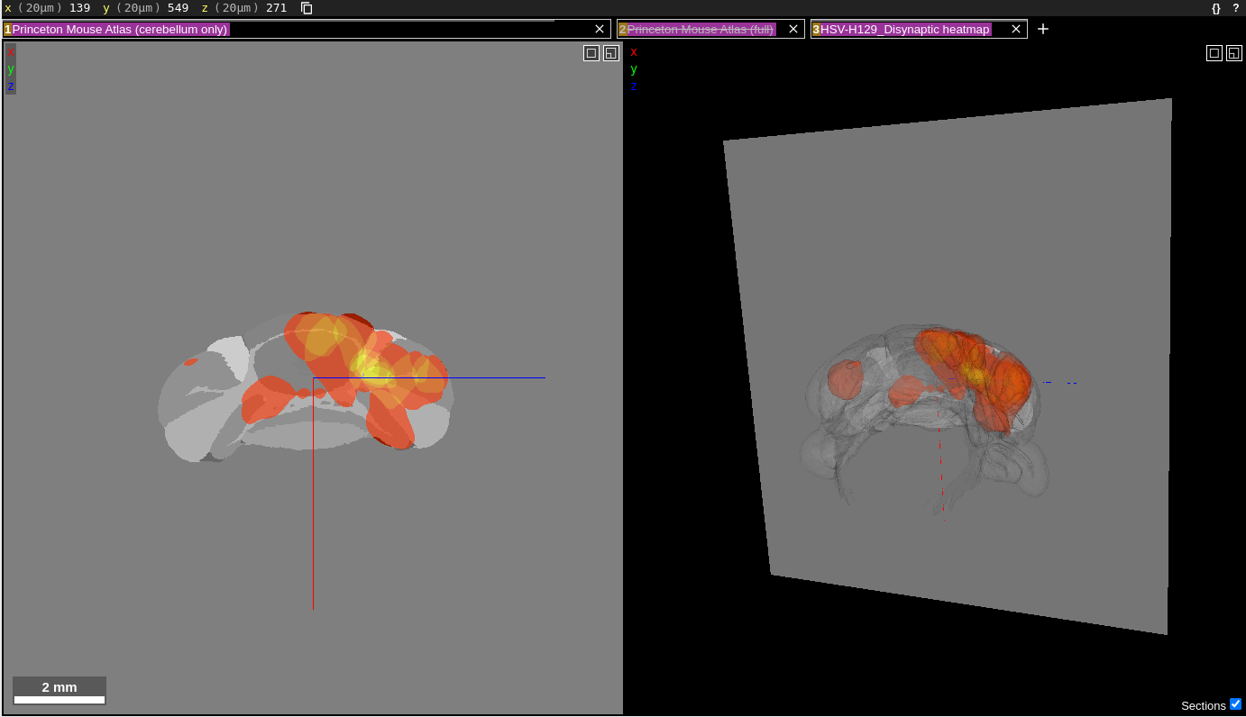
The “Princeton Mouse Atlas (cerebellum only)” is the first layer in the layer list. This layer shows the individual regions comprising the cerebellum in grayscale. The second layer in the layer list is the “Princeton Mouse Atlas (full)”, which is disabled, as indicated by the strikethrough text in that layer box. When enabled, this layer shows the individual regions of the entire Princeton Mouse Atlas. The third and final layer is the heatmap of injections for the HSV-H129 Disynaptic timepoint. Layers can be toggled on/off by clicking anywhere in the corresponding text box for that layer. Once disabled, the layer text will contain a strike through its name. Clicking the “x” in a layer box will remove that layer from the visualization.
The data are displayed in a 2D coronal view (left panel) and a 3D view (right panel). The two panels are synced together; the gray plane in the 3D view corresponds to the section shown in the 2D view. There is also an x,y,z coordinate axis (blue, red, green lines) that indicates the center of both views. It can be used to determine the relative orientation between the two views.
Some basic commands for exploring the data are as follows:
- h key: open help menu
- (2D view) left-click and drag: translate section
- (2D and 3D view) mouse-wheel: scroll along anterior-posterior (AP) axis.
- (2D and 3D view) shift+mouse-wheel: scroll (x10 speed) along anterior-posterior (AP) axis.
- (2D and 3D view) ctrl+mouse-wheel or ctrl+”+/-“: zoom in and out
- (2D and 3D view) double left-click: select/de-select segment
- (2D and 3D view) Hover over a segment: highlights the region and displays the brain region name in the atlas layer box area.
- (3D view) left-click and drag: rotate brain
- (3D view) s key: toggle the gray reference slice on/off
- right click on layer box: open up options for displaying that layer such as opacity, color scheme, segment selection
Finally, the neuroglancer URL is updated in real time each time you make a change to the viewer. If you reach a state that you want to save and share, simply copy the neuroglancer URL from your browser. If you want to restore to the original state, come back to this page and click the link again.
Injection site heatmaps
The following three links display synced 2D and 3D heatmaps overlaid on the Princeton Mouse Atlas. Each link shows the heatmap at a different timepoint. The color of the heatmap indicates the number of brains injected at that location. When hovering over a region of the heatmap, the number of brains injected at that location is displayed in the heatmap layer box, which is the last in the layer list at the top of the screen.
HSV-H129 Disynaptic timepoint (heatmap) an012 HSV-H129 Trisynaptic timepoint (heatmap) an012 PRV Disynaptic timepoint (heatmap) an012Injection volumes separated by primary injection site
The links below show the volumetric injection sites for individual brains, organized by primary injection site. We categorized the primary injection sites into seven distinct brain areas in the cerebellum:
- Paramedian lobule, Copula Pyramidis
- Lobule I-V
- Lobule VI, VII
- Lobule VIII-X
- Crus I
- Crus II
- Simplex
For each primary injection site heading below, there are links for each of the three timepoints. When the links are first loaded, the injection sites from all brains having the given primary injection site at the given timepoint are displayed in the same color on top of the Princeton Mouse Atlas. The layer box at the top with “pooled_by” in the name contains this data.
The remaining layers consist of the layer boxes with names “… 01”, “… 02”, and so on. These layers show the injection sites for the individual brains in different colors. These layers are all disabled by default.
Paramedian lobule (PM), Copula Pyramidis (CP) injections
HSV-H129 Disynaptic (PM, CP) an012 HSV-H129 Trisynaptic (PM, CP) an012 PRV Disynaptic (PM, CP) an012Lobule I-V Injections
HSV-H129 Disynaptic (Lob. I-V) an012 HSV-H129 Trisynaptic (Lob. I-V) an012 PRV Disynaptic (Lob. I-V) an012Lobule VI, VII injections
HSV-H129 Disynaptic (Lob. VI, VII)HSV-H129 Trisynaptic (Lob. VI, VII)
PRV Disynaptic (Lob. VI, VII)
Lobule VIII-X injections
HSV-H129 Disynaptic (Lob. VIII-X) an012 HSV-H129 Trisynaptic (Lob. VIII-X) an012 PRV Disynaptic (Lob. VIII-X)Crus I injections
HSV-H129 Disynaptic (Crus I)HSV-H129 Trisynaptic (Crus I)
There were no injections for the PRV Disynaptic timepoint in Crus I
Crus II injections
HSV-H129 Disynaptic (Crus II)HSV-H129 Trisynaptic (Crus II)
PRV Disynaptic (Crus II) an012
Simplex injections
HSV-H129 Disynaptic (Simplex) an012 HSV-H129 Trisynaptic (Simplex) an012 PRV Disynaptic (Simplex)Jupyter notebooks to reproduce or customize these Neuroglancer visualizations can be found here: https://github.com/PrincetonUniversity/lightsheet_helper_scripts/tree/master/projects/tracing/injection_site_neuroglancer_post/notebooks
The Python interface to Neuroglancer
The Python interface to Neuroglancer provides several advantages over using fixed links to your data, such as the visualization links generated at the braincogs00.pni.princeton.edu site. The main advantage is that it gives you programmatic control over your Neuroglancer session. A popular use case is for making reproducible figures and movies via the screenshot feature. It also allows you to keep the Neuroglancer session open indefinitely, whereas the links on braincogs00 expire after a few hours of inactivity. If you are making annotations for longer than a single sitting, you could lose your progress if the Neuroglancer session is closed while you are away from your computer. By using the Python interface, you don’t have to worry about that happening.
A tutorial on how to start using the Python interface to Neuroglancer is written up here: https://github.com/PrincetonUniversity/lightsheet_helper_scripts/blob/master/neuroglancer/neuroglancer-python_tutorial.ipynb. The basic idea is you boot up a jupyter notebook and make a connection to a Neuroglancer session. As long as the jupyter notebook is running, the connection to Neuroglancer will remain open. Here is what is covered in the notebook:
- Start a Neuroglancer session from Python and load in public data
- Manipulate the Neuroglancer session from Python
- Add custom annotations to Neuroglancer using Python
- Configure and take a screenshot and movie reproducibly
- Load in private light-sheet data from bucket
There is a lot more that can be done with the Python interface, such as defining your own keyboard shortcut that executes a custom Python program. We will explore this feature in a future post.
Displaying atlas region boundaries in Neuroglancer
We recently added the three dimensional atlas developed by Chon et al. 2019 (PI Yongsoo Kim; Penn State; https://www.nature.com/articles/s41467-019-13057-w) as an option to which we can register your mouse brain light sheet images using our automatic brain registration pipeline, BrainPipe. This atlas merges the widely adopted Franklin-Paxinos (FP) labels into the Allen Institute’s common coordinate framework (CCF). By aligning your data to this atlas, you can overlay the FP boundaries on your light sheet data as shown below. This atlas is only suitable for coronal slice viewing (the resolution is poor in the horizontal and sagittal views). The atlas consists of 123 coronal slices (100 micron spacing), with a spatial resolution of 10×10 microns in each coronal plane.
If you are used to viewing our previous atlases in Neuroglancer, you will notice that this looks a bit different. In the past, we have visualized atlases using the “filled” multi-color format:
Showing the boundaries of regions is possible for all of the brain atlases, not just the FP atlas. We store the boundaries in a separate segmentation layer, so in order to see the boundaries this layer needs to be loaded just like an ordinary atlas layer. The Allen, Princeton and FP atlas boundary segmentation layers are all publicly available on our google cloud bucket: gs://wanglab-pma. To load the FP boundary layer into Neuroglancer, for example, type this into the source box:
precomputed://gs://wanglab-pma/kimatlas_boundaries/
If you only load in the segment boundary layer for an atlas, the region name will only appear in the top layer box when you are hovered over the actual boundary. Below is a short video demonstration of what I mean. The region name will appear in the green rectangle (the layer box) near the top of the screen only when the segment is highlighted.
Many people find this inconvenient and prefer for the region name to be displayed if you are hovered anywhere inside of a region. If you are one of these people, a trick is to load the original “filled” atlas layer and then turn the transparency of this layer down, like so:
Like with all segmentation layers, you can select individual segment boundaries either manually by double clicking them, using the search tool described in one of our previous posts, or via the Python API.
As usual, if you have any issues are questions feel free to let us know at ahoag@princeton.edu or lightservhelper@gmail.com.
Using the Neuroglancer search/filter tool
There are several ways to select which segments to display in Neuroglancer. One we have already covered in the “Getting Started with Neuroglancer” post is double clicking individual segments to select them. This works well if you already know exactly where the segment is and you only have a few segments. Note: in this post “segments” refers to brain regions, and I will use segments and regions interchangeably.
In cases where you have many regions or you don’t know exactly where a region is by memory, Neuroglancer offers a powerful search feature*. This allows you to filter which brain regions you want to display by pattern matching against the segment name or ID. The search tool can be found in the “Seg.” tab in the control panel on the right hand side of the screen (which can be opened via ctrl+click on the layer name at the top). Note that the tool is only available for segmentation layers (e.g. brain atlases). The following figure shows how to locate the search tool.
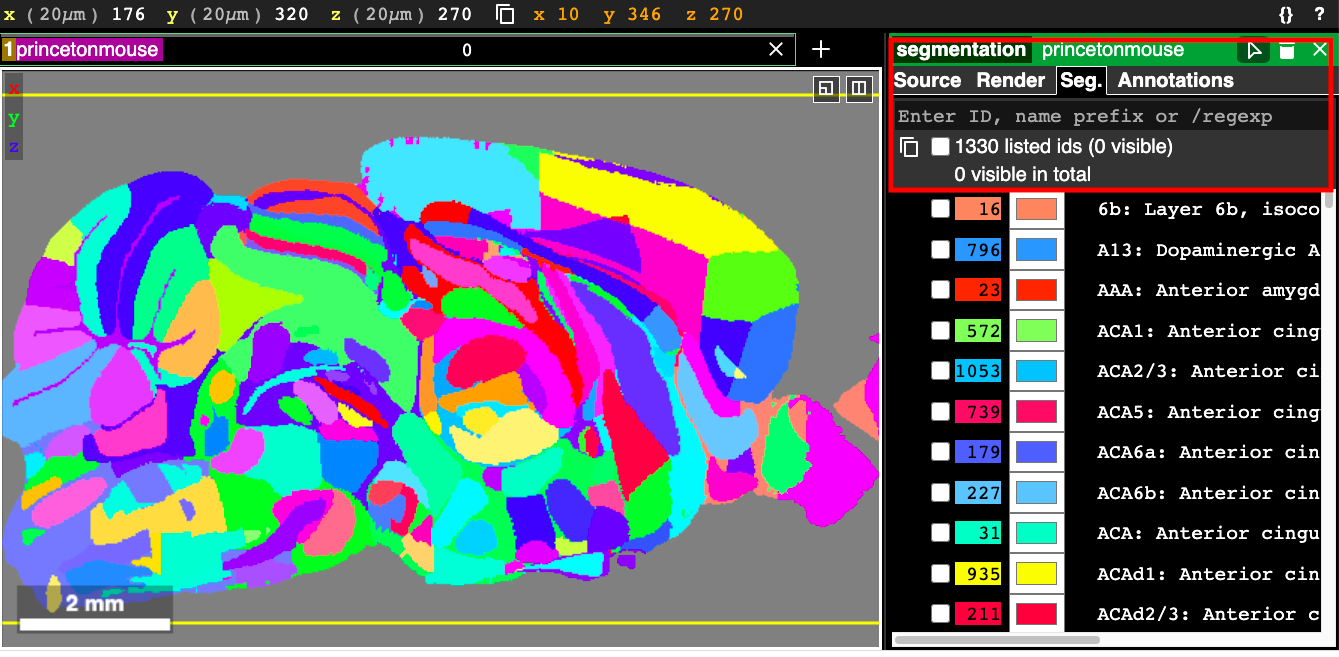
When nothing is entered in the search tool, the text that is displayed gives us some instructions: “Enter ID, name prefix or /regexp”. This explains the three ways you can filter segments. Each segment has an integer ID, shown in the list of segments below the search box in the above figure, and you can simply enter in the ID to select just that region. You can select multiple segments by entering in a comma-separated list of IDs, like in this example:
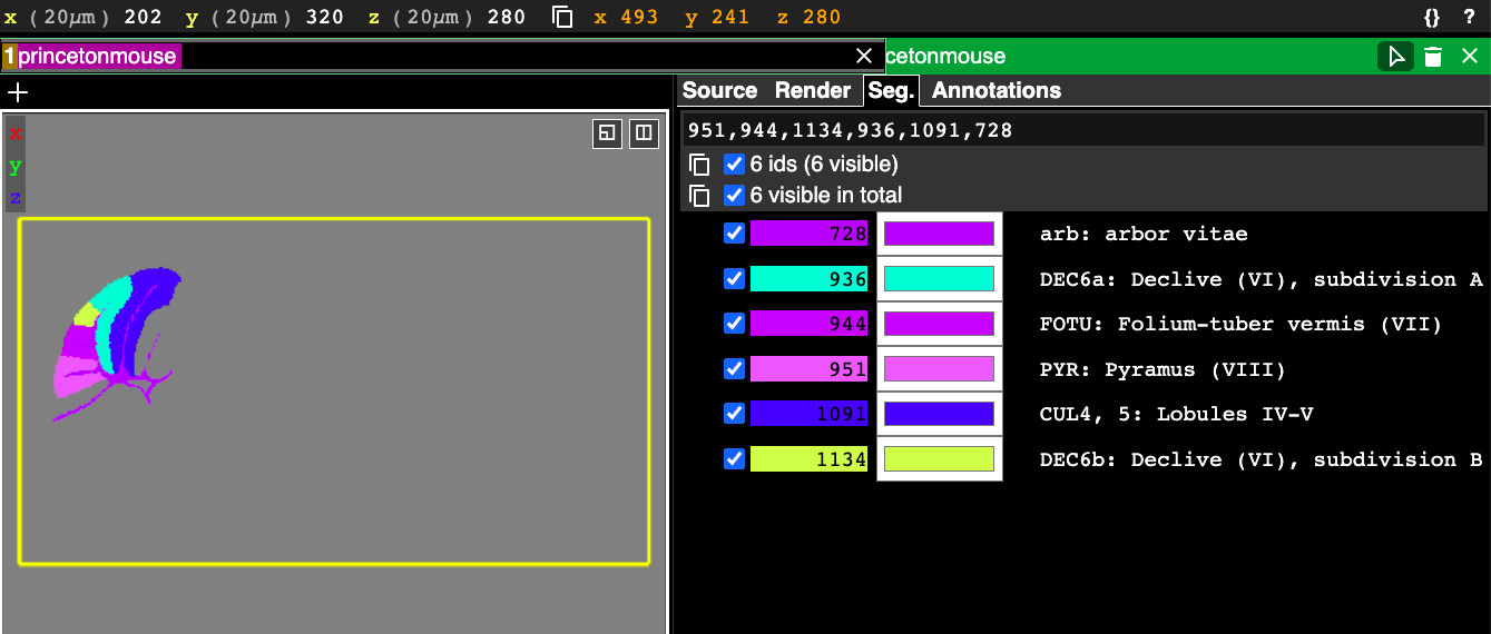
It is often much more convenient to search by region name or acronym than by this somewhat arbitrary integer ID. Notice in the above figure that each selected segment has an entry in the right hand side panel showing the id, color, and the acronym, followed by the full name of the segment. This text here can be used in the search as well.
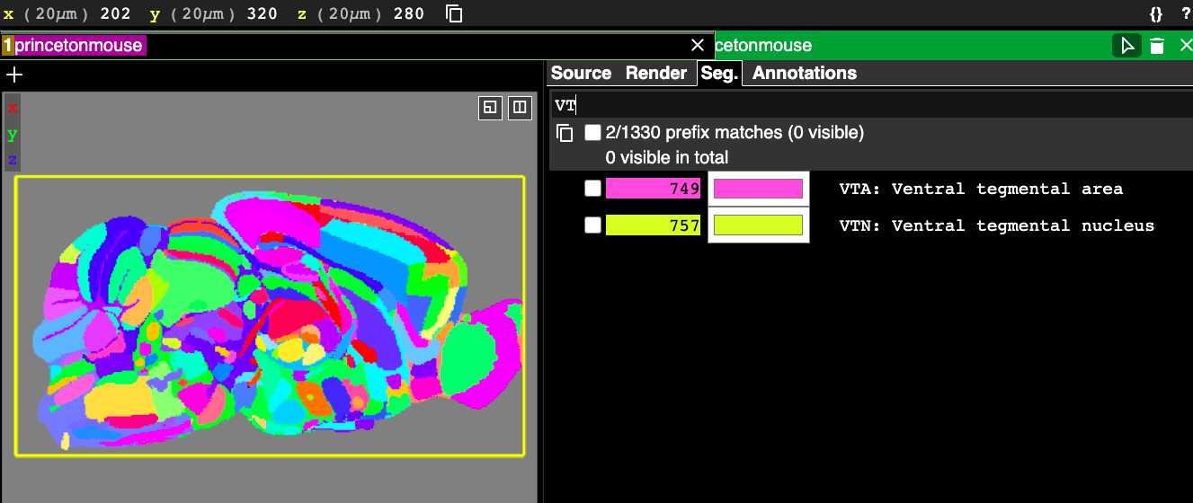
The first way to filter based on text is using the “name prefix”. To do this, you just start typing some text and whichever segments’ text begins with what you’ve typed appears in the segment list below and can be selected. Note that it is case sensitive. In the following example I start typing VT and two matches appear because there are two acronyms in the Princeton Mouse atlas that start with “VT”, which are the VTA and the VTN.
The final way to search is the most powerful and arguably the most useful. This is using the “/regexp” feature, which stands for “regular expressions” (sometimes just called “regex”). Regular expressions are “a sequence of characters that define a search pattern” according to wikipedia: https://en.wikipedia.org/wiki/Regular_expression. Here is a description of some of the special characters that regex uses with interactive examples: https://www.w3schools.com/python/python_regex.asp. It is not necessary to be an expert in regex to use it effectively in Neuroglancer, but knowing a little about some of the special characters it uses can go a long way.
Before diving into regex use cases, it is a good idea to analyze the format of our segment text labels. Understanding the format will help us pattern match using regex much more effectively. Looking at the above figures, note that the segment labels seem to always start with an acronym, following by a “:” then a space, followed by the full region name. The first word after the “:” is usually capitalized, but it is not always as in the example: “arb: arbor vitae”.
Let’s say we want to find a specific brain region, the “mediodorsal nucleus of thalamus” without knowing its acronym or which words if any are capitalized. If we just start typing “mediodorsal” in the search box there are no matches. That is because the search tool by default always tries to match the beginning of the region string, which for this atlas always starts with the acronym. To search for a word within the entire region string but not necessarily at the beginning, we need regex.
To activate the regex, you need to put a “/” before the pattern you are searching for. By typing /mediodorsal this means “search for any instance of the all-lowercase string ‘mediodorsal’ in the entire segment text string”. After typing this in you will see a match, but it’s not the right one. The match is to the region: “IMD: Intermediodorsal nucleus of the thalamus”, where I have bolded the part that gets matched. The regex search is case sensitive. To make the search case insensitive use the regex /[Mm]ediodorsal, where “[Mm]” means match “either M or m”, then match the rest of the word as all lowercase. With this new query you get five matches, including the one we’re after: “MD: Mediodorsal nucleus of thalamus”.
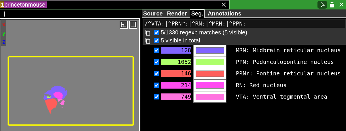
Let’s consider another example where we have a list of five acronyms for regions that we want to show at the same time. We’re not completely sure what the full names of the regions or the IDs they correspond to are. Let’s say these acronyms are: VTA, PRNr, RN, MRN, PPN. We know these will come at the beginning of each match, so we can use the special “^” regex character before our acronym to enable that. We also know that the acronym ends with a literal “:”. This is important to include because if we don’t, searching for RN could match an acronym that starts with RN but has more characters. Finally, we can use the “|” (the regex OR operator) to match multiple acronyms in the same query. The full regex to match all five of these regions using only their acronyms is: /^VTA:|^PRNr:|^RN:|^MRN:|^PPN:. Here it is in action:
Note that not all atlases are guaranteed to have acronyms. We customized the region labels for this atlas to include the acronyms, but other atlases may not even have acronyms. Again, it is a good idea to look at how your segment labels are generally formatted when coming up with the right regex query.
With just a few basic regex operators we are able to achieve a lot of search power. There are many more regex operators (see links above), but we will only discuss one final one, the end of line matching operator, “$”. This is useful if you know the full region name but not the acronym. For example, let’s try to match the region “TH: Thalamus”, but say we don’t remember the acronym. Based on what we have covered so far we might try “/[Tt]halamus”. If we do that, we see 50 matches. No so helpful. If we tack on a “$” at the end of the query: /[Tt]halamus$, then this says “match the word thalamus with a captial or lowercase T and with the word appearing at the end of the string.” This query narrows it down to 36 matches, which is slightly better, but there is one more piece we need. Since we know thalamus is the only word in the region, it must come after its acronym. While we don’t know what the acronym is, we know the “:” character follows the acronym and there is a space between “:” and the first word of the region name. So if we change our regex to: /: [Tt]halamus$, then we get a single match, and it is the one we want: “TH: Thalamus”.
One final thing to note is that if you are fond of using the Python API for scripting your Neuroglancer sessions the segment query can be applied programmatically. This jupyter notebook example demonstrates how to do this: https://github.com/PrincetonUniversity/lightsheet_helper_scripts/blob/master/neuroglancer/segment_query_tutorial.ipynb
Hopefully this gets you started with using the search tool. Let us know if you find novel ways to use the search regex or have any questions!
* The search feature is available in the Google Neuroglancer client (https://neuroglancer-demo.appspot.com) and BRAIN CoGS Neuroglancer client (https://nglancer.pni.princeton.edu), but may be absent or function differently in other clients.
New Neuroglancer feature: import annotations from CSV files
Annotations are a useful feature of Neuroglancer. In previous posts, we’ve gone over how to add annotations to mark regions of interest in our lightsheet volumes. In the Brain Registration and Histology Core Facility at PNI, we also frequently use annotations to display detected cell locations. In cases like this, where we want to create lots of annotations and we already know their locations in our volume, it is very tedious to manually add them. The goal of this new feature is to provide a more convenient way to upload many annotations simultaneously.
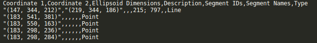
This is now possible using the “Upload from CSV” button. This screenshot shows the required format of the uploadable CSV file.
The video below explains the formatting of this file as well as some other features of the new import csv button.
Note that importing annotations from a CSV file is not efficient for very large numbers of annotations. If you start noticing that loading your CSV file is taking a while (usually for ~10^4 or more annotations), you may want to consider a second method for getting the annotations into Neuroglancer. This other method involves creating a precomputed annotation layer and then hosting the layer. This method can load up to 10^7 annotations in less than a second. This method is a bit more work and is not covered in this post, but it will be covered in a future post. Feel free to reach out in the meantime if you want to explore this method.
Visualizing different levels of the brain atlas structure hierarchy graph in Neuroglancer
Brain atlases, such as the Allen Mouse Brain Atlas (AMBA) and Princeton Mouse Brain Atlas (PMA) are invaluable tools. They allow data from different experiments to be compared and analyzed in the same framework. With Neuroglancer and other visualization tools, they allow data to be visualized in the same framework as well.
The way we visualize these atlases with Neuroglancer is by showing their atlas annotation volume. Described here for the AMBA, the annotation volume is a 3D volume containing ids at voxels corresponding to the locations of brain regions. Each id represents a different brain region. When the Allen Brain Institute created their annotation volume, they had to choose what level of brain divisions to use. For example, did they want to display only the very large brain divisions like Cerebral Cortex, Cerebellum and Brain Stem, or the more detailed subdivisions such as the nuclei contained within these larger regions? Allen largely chose the latter option, which is why their annotation volume has so many small regions:
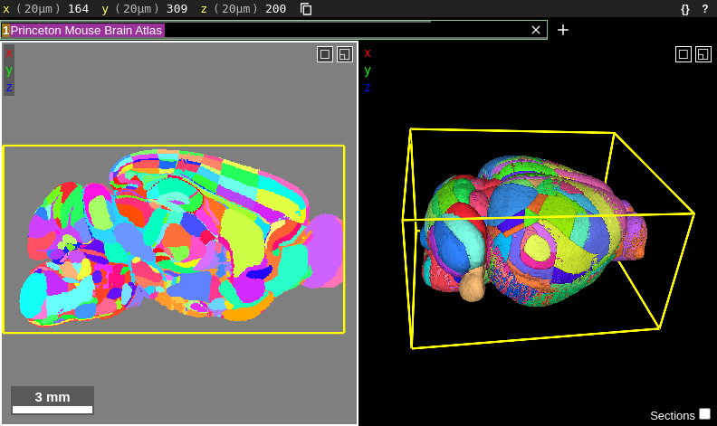
But what if the researcher wants to display larger brain divisions for a figure they are making? Fortunately, we are not stuck with visualizing the atlas only at the brain divisions that Allen chose. To figure out how to overcome this, we need to understand the atlas structure hierarchy (sometimes referred to as the “brain ontology” or “structure ontology”). The structure hierarchy is a set of parent-child relationships describing how the large and fine divisions of the brain are related. They are nicely visualized using directed graphs. For example, here is the structure hierarchy graph for the Striatum, a brain region situated beneath the cerebral cortex in the mammalian brain that is critical for many cognitive functions. Hover over the image to zoom. Clicking the image will open it in its own window.
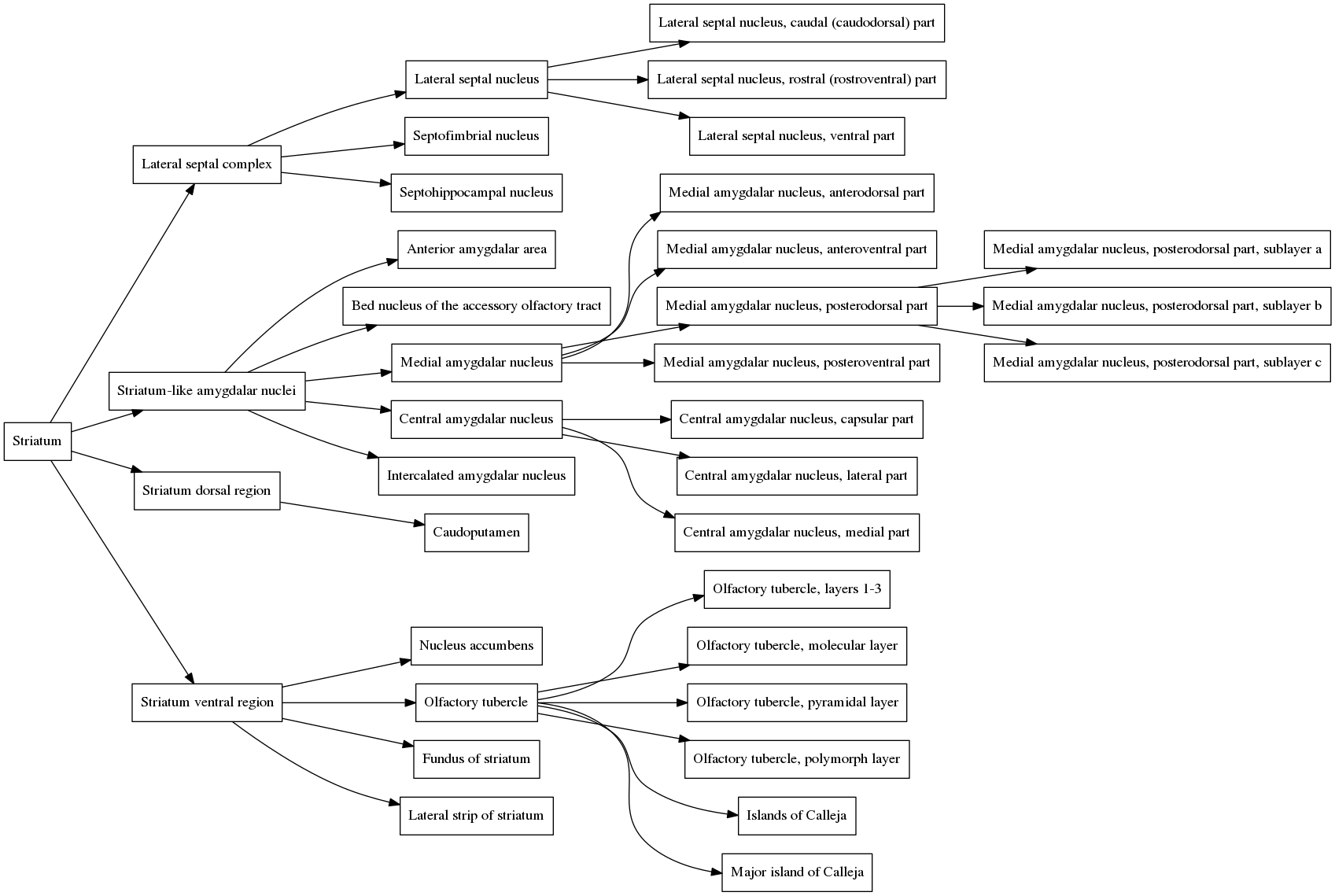
In the graph, the Striatum is the parent node (all the way to the left). It is composed of four smaller regions, the Lateral septal complex, the Striatum-like amygdalar nucleus, the Striatum dorsal region and the Striatum ventral region, all of which are connected to the Striatum by edges in the graph. Each of these subregions is composed of its own set of subregions, which themselves have subregions, and so on. The entire brain can be organized in this way, and the structure hierarchy defines all of these relationships. The graph of the structure hierarchy of the entire mouse brain is massive and impractical to show on this page, but we don’t need it to understand how the structure hierarchy is organized.
So what we need to do in Neuroglancer if we want to show larger brain divisions than Allen’s defaults is to modify the structure hierarchy that the annotation volume is using. I created a key binding in Neuroglancer that allows users to do exactly that. One key (“p” for parent) allows users to go up a level in the hierarchy, and another key (“c” for child) allows them to go in the opposite direction. It makes use of Neuroglancer’s segment equivalences feature by merging children with their parents so they have the same color and id. Here is a video example showing these key bindings in action for the Striatum. At the beginning of the video, the default structure hierarchy of just the Striatum is displayed, corresponding to the graph shown above. The “p” key is pressed three times, showing the structure hierarchy collapsing to larger and larger divisions until the entire Striatum is shown as a single region. At the end of the video, the “c” key is pressed and the original divisions are restored.
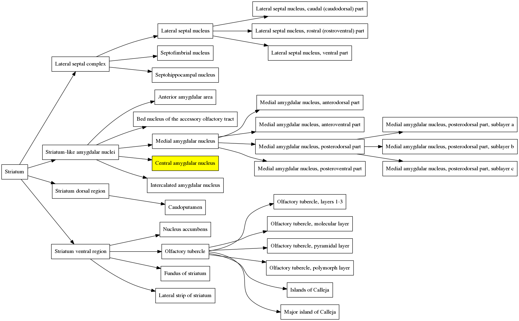
Here is the an illustration of what is happening in the structure hierarchy graph when the atlas is contracted in the video above. Immediately before the atlas is contracted the first time, the cursor is on the brain region: “Central amygdalar nucleus, capsular part”, which is highlighted in the graph below to show which branch we are in.

When the atlas is contracted the first time, this region and its siblings are merged with the parent region, the “Central amygdalar nucleus”. That branch in the structure hierarchy graph therefore gets one level smaller and is now:
When the atlas is contracted a second time, all of the siblings of the “Central amygdalar nucleus” and all of their descendants get merged with the parent, the “Striatum-like amygdalar nuclei”, and the graph becomes much simpler:
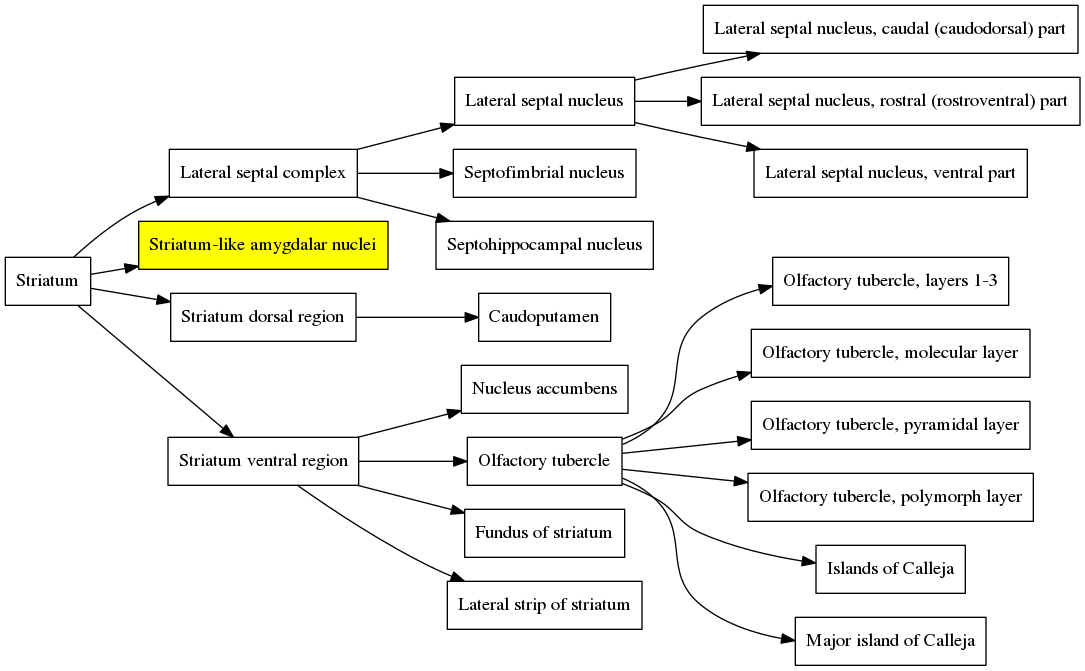
And finally when the contraction is performed again, the entire structure collapses back to the Striatum because the “Striatum-like amygdalar nuclei” is a child of the Striatum and therefore all of its siblings are also children of the Striatum. So the graph simply becomes:

At the end of the video the “c” key is pressed and the original structure hierarchy of the Striatum is restored.
A jupyter notebook walking through how I created these graphs and the Neuroglancer add-on is available here: https://github.com/PrincetonUniversity/lightsheet_helper_scripts/blob/master/neuroglancer/merge_ontology_tutorial.ipynb
Try out the tool yourself in this live demo (only available within the Princeton network of VPN): https://braincogs00.pni.princeton.edu/neuroglancer/merge_ontology_demo
Princeton Mouse Brain Atlas links
Interactive 2D/3D Neuroglancer volume: https://brainmaps.princeton.edu/pma_neuroglancer
Atlas tissue volume: https://brainmaps.princeton.edu/pma_tissue
Atlas annotation volume: https://brainmaps.princeton.edu/pma_annotations
Atlas id to name mapping: https://brainmaps.princeton.edu/pma_id_table
Atlas structure ontology list: https://nbviewer.jupyter.org/github/PrincetonUniversity/lightsheet_helper_scripts/blob/master/projects/combine_cfos_batches/data/PMA_regions.html
These files are shared under the CC BY-NC-ND license (https://creativecommons.org/licenses/by-nc-nd/4.0/).
Probe Detection Example with Neuroglancer
One of the common use cases of the light sheet microscope at PNI is post-experiment validation of the anatomical location of a probe inserted into a rodent brain for neural recording. The following video illustrates via example how to use the tools in Neuroglancer for probe detection and annotation.